An ordinary day
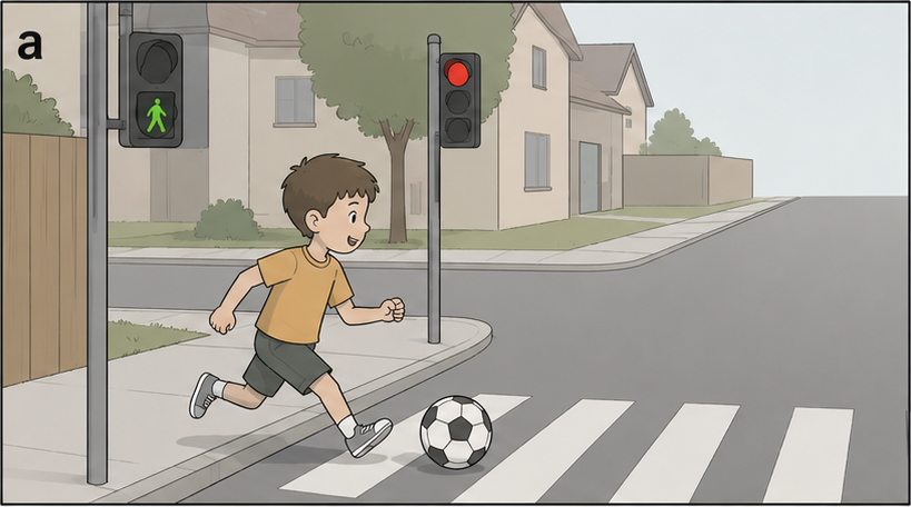
A child runs after a ball. The crossing looks like every other crossing; nothing suggests danger.
So that rare events are neither ignored nor over-amplified.
Where everything starts
How brains build accurate internal models from limited experience is a central question in neuroscience.
A child runs after a ball. The crossing looks like every other crossing; nothing suggests danger.
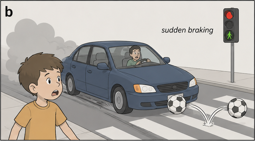
The child is almost hit by a rushing car.
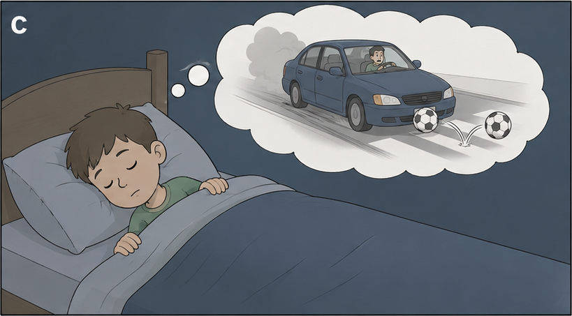
At night the scene comes back. The brain replays what it saw and rehearses what it might see again.
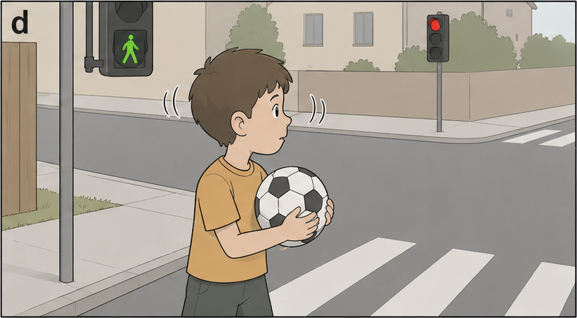
The child holds the ball at the kerb. A single memory has changed a lifetime of predictions.
The same near-miss, three internal models of how likely it is to happen again.
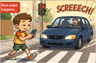
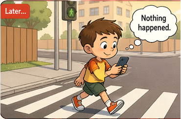
The event is filed away as a one-off. Next time the child walks out just the same.
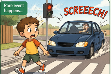
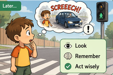
The event is rare but real. It is remembered, replayed, and acted on when it matters.
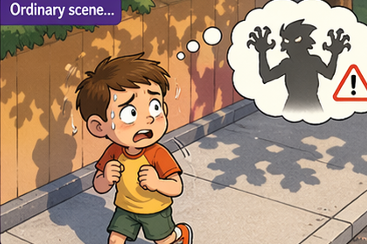
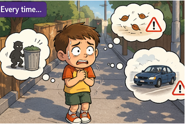
The event colours every scene. Ordinary streets now feel dangerous.
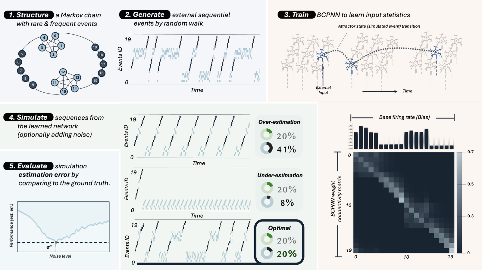
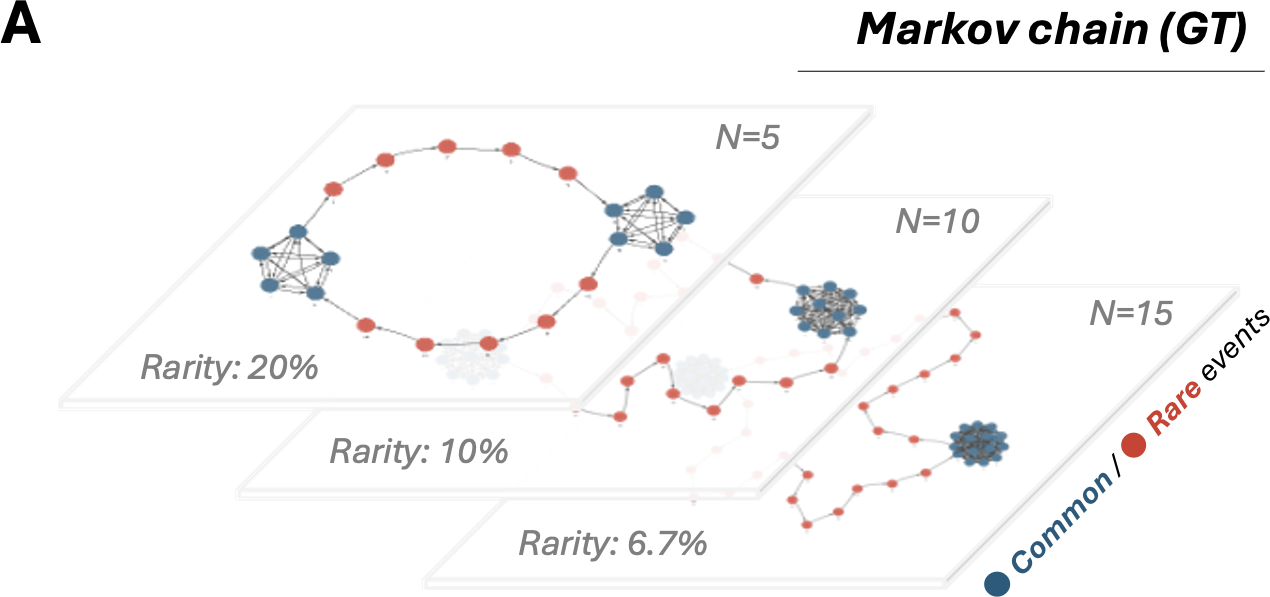
A Markov chain is the ground truth. The network must build an internal model of it from limited samples, and get the rare transitions right.
(A) The ground-truth (GT) Markov chain, shown at three rarity levels (N = 5, 10, 15; rare share 20%, 10%, 6.7%); common/rare events are blue/red.
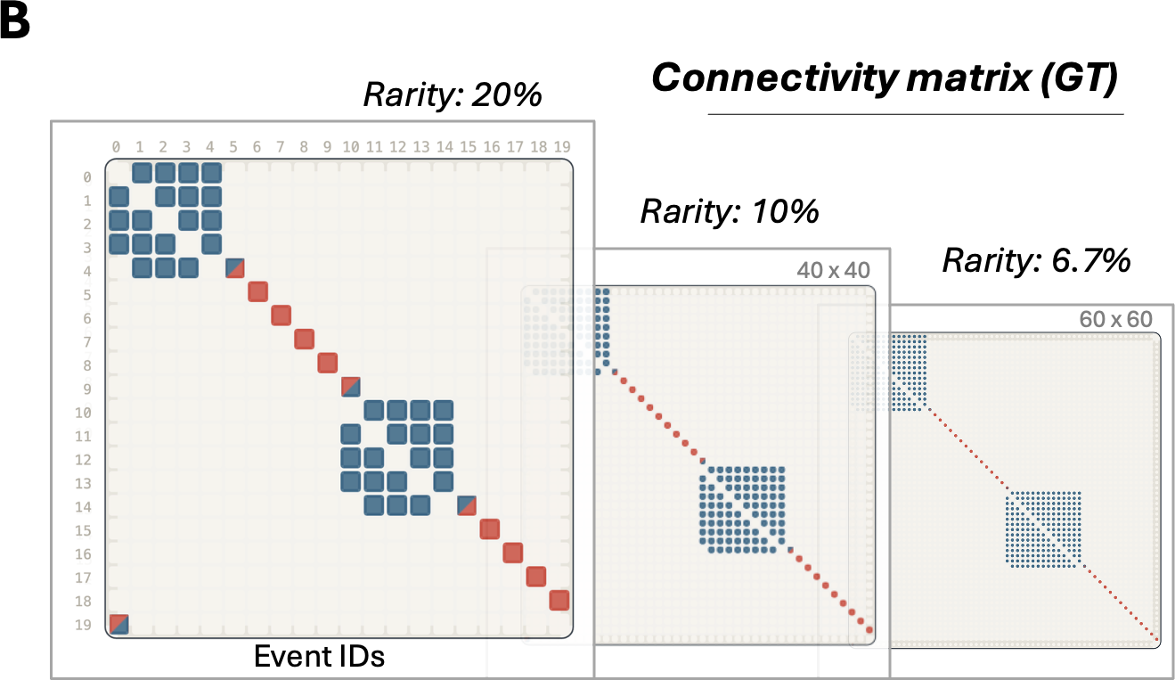
(B) The GT connectivity matrix; dense diagonal blocks (blue) mark common cliques, and sparse red entries mark rare chains.
(C) Per-event stationary probability, the marginal occurrence; the dashed threshold refers to GT occurrence of a rare event.
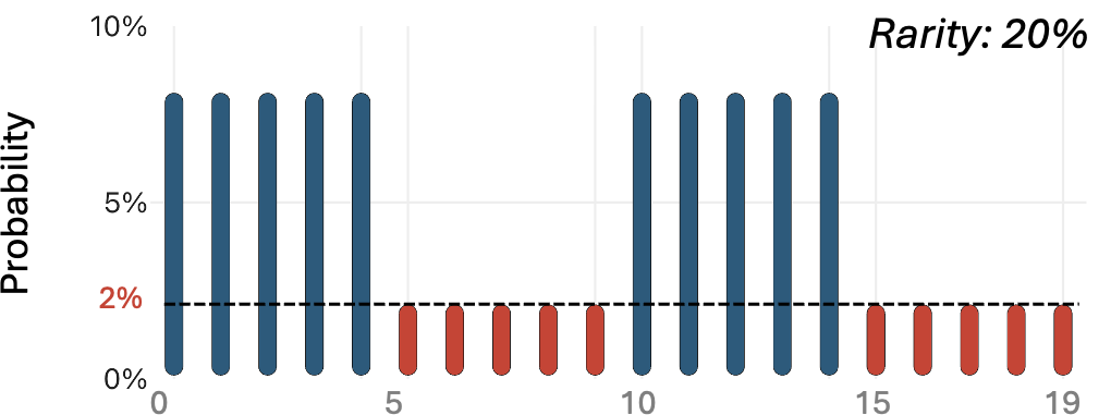
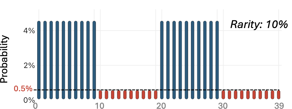
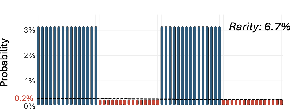
Change the chunk size and watch the chain, its connectivity matrix and the per-event probabilities update together.
How sequences are generated from the Markov chain, and how performance is measured.
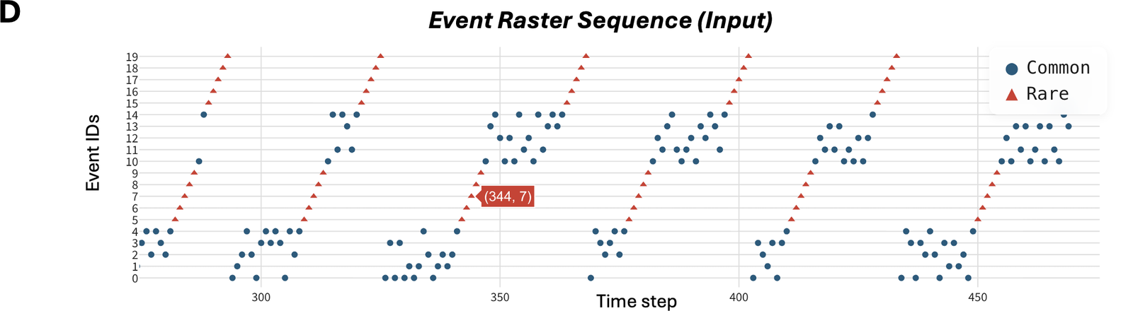
(D) A representative input sequence, shown as an event raster.
(E) Level-1 (marginal) occurrence: the common and rare occurrence shares are shown, with the GT rare share marked by the dashed line, and the signed occurrence deviation from the GT is displayed over time, upward red markers denoting over-representation (> 0) and downward blue markers under-representation (< 0).
(F) Level-2 (conditional) occurrence: the four transition-type occurrences are displayed for the input against the GT (translucent), and their occurrence divergence, a KL divergence, is shown over time. Definitions are given in Methods.
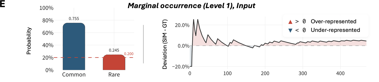
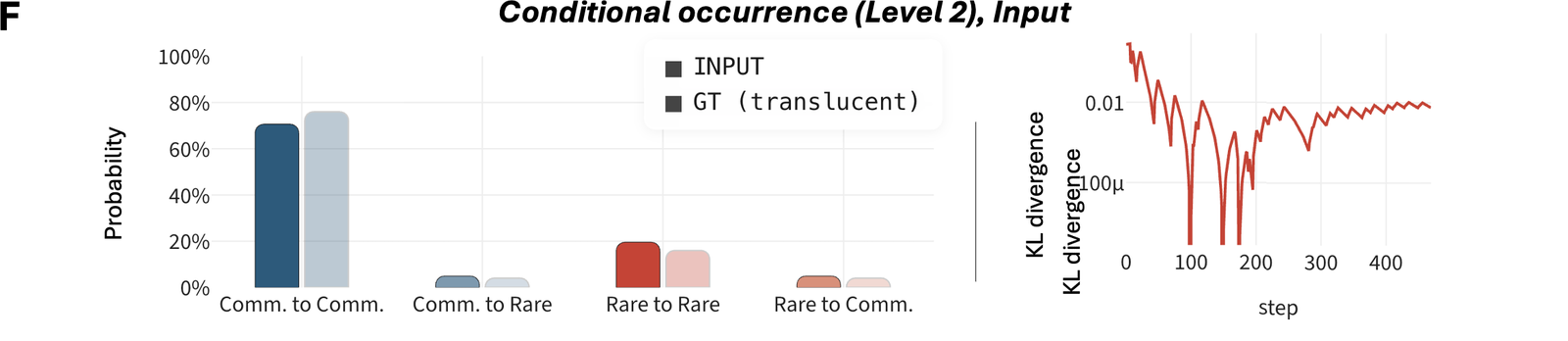
A random walker on the ground-truth chain produces this sequence step by step, with the raster and both measurement levels updating live.
The internal model. A Bayesian Confidence Propagation Neural Network, biologically plausible attractor dynamics with local Hebbian / Bayesian learning. Each unit holds a support value, an intrinsic bias (log-prior), and synaptic weights that update from co-occurrences. After learning, the network runs autonomous replay driven by these parameters alone.
One cortical minicolumn, about 100 tightly interconnected neurons, is treated as one computational unit. Minicolumns group into hypercolumns, where local competition turns their activities into a probability distribution over one attribute.
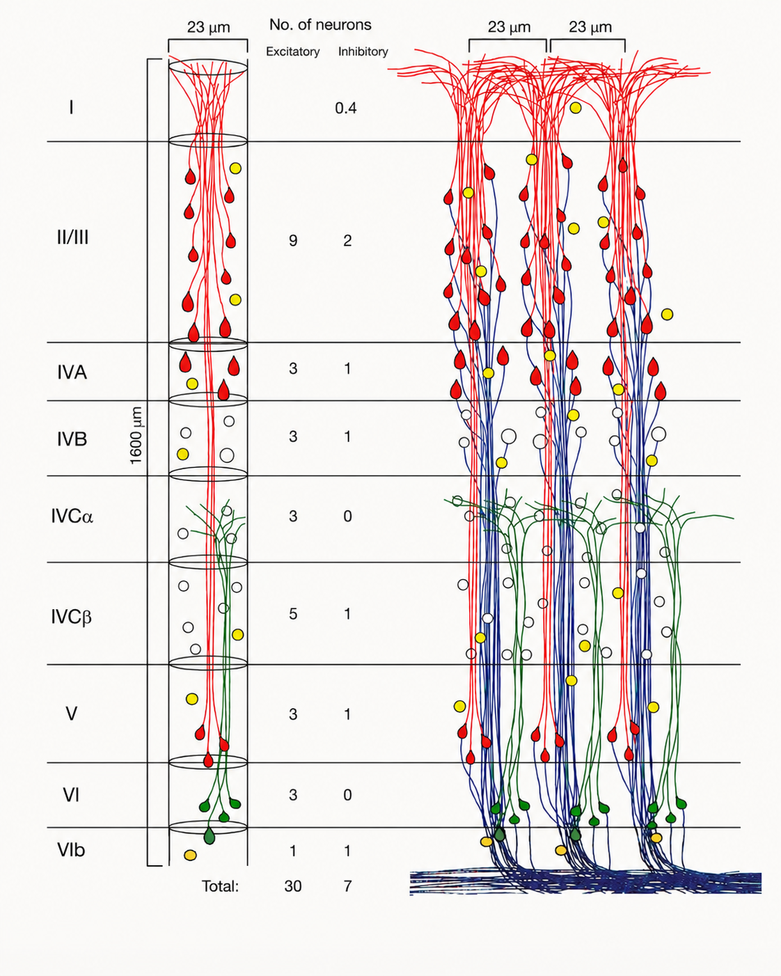
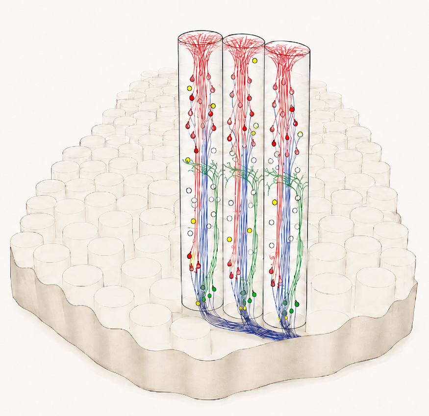
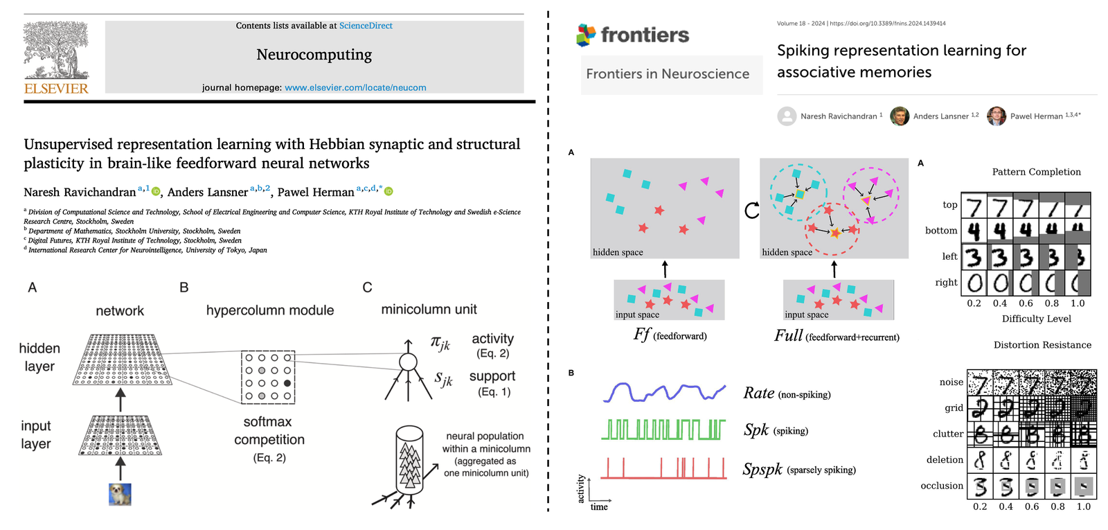
With Hebbian-Bayesian plasticity the same network learns spatial correlations, giving pattern completion under noise, and temporal order, letting it replay learned sequences from its own connectivity.
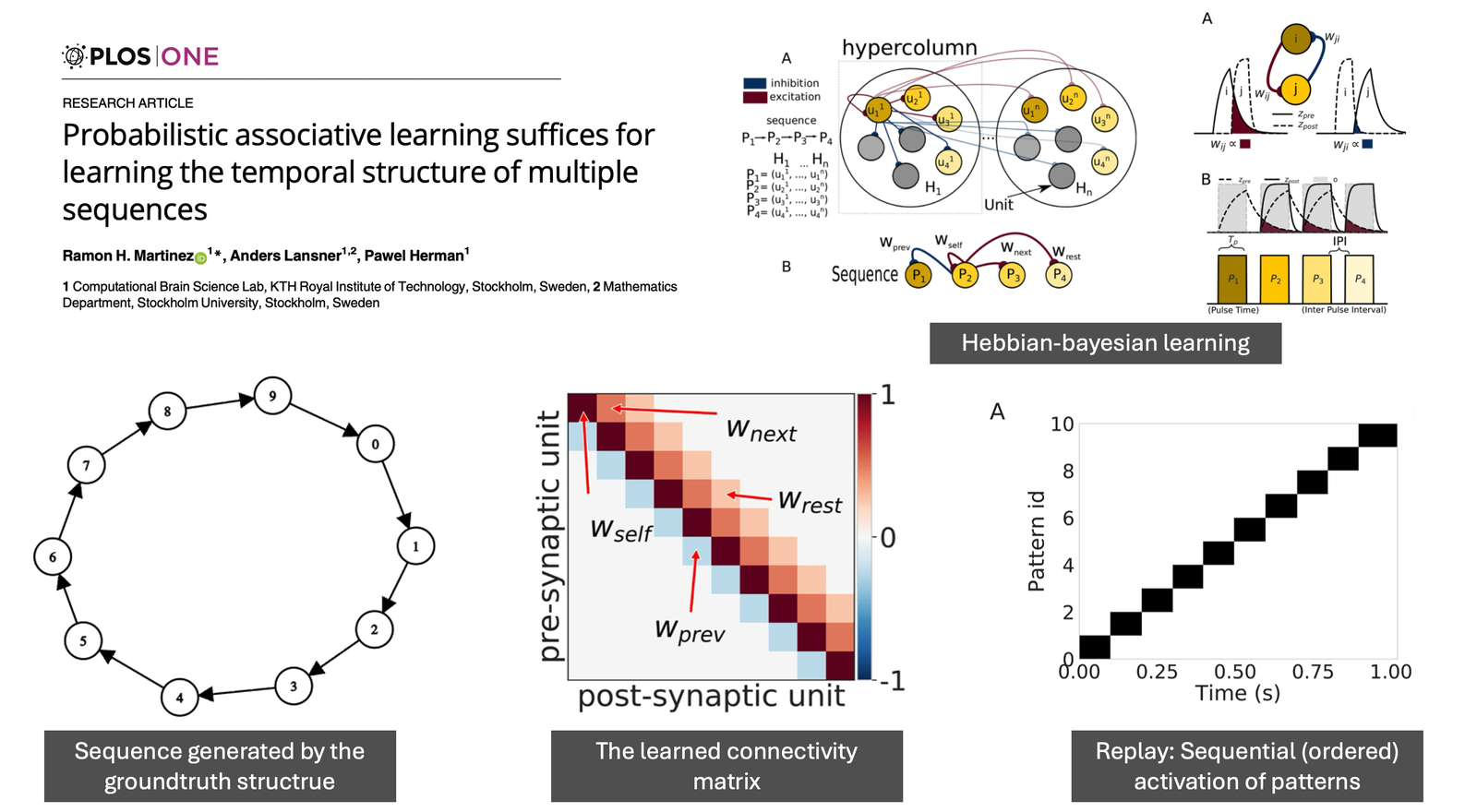
During training, Hebbian plasticity converts the externally driven firing sequence into directed synaptic weights between units. During recall, no external drive is needed, and one minicolumn's firing propagates through its strongest learned synapse to the next, traversing the entire chain from a single seed cue[8].
The BCPNN learns by estimating probability distributions from data, then turns those estimates into synaptic weights and biases. The six equations below specify the model.
Support — total drive into a unit (lateral input + bias + external cue + noise), low-pass filtered with time constant $\tau_s$:
$$ \tau_s \frac{ds_j}{dt} = \beta_j + \sum_i w_{ij}\, o_i - s_j + G_I\, I_j(t) + \sigma(t) $$
Output — softmax (winner-take-all) across the units of one hypercolumn, sharpness $K$:
$$ o_j = \frac{e^{K s_j}}{\sum_i e^{K s_i}} $$
Marginal probability — running estimate of how often unit $j$ is active, with slow time constant $\tau_p$:
$$ \tau_p \frac{dp_j}{dt} = o_j - p_j $$
Joint probability — running estimate of how often units $i$ and $j$ co-fire (Hebbian trace):
$$ \tau_p \frac{dP_{ij}}{dt} = o_i\, o_j - P_{ij} $$
Synaptic weight — log-ratio of joint to independent probability (pointwise mutual information):
$$ w_{ij} = \log\!\frac{P_{ij}}{p_i\, p_j} $$
Bias — log-prior probability of the unit:
$$ \beta_j = \log p_j $$
The weight rule is online and local: each synapse needs only its pre- and post-synaptic activity. The softmax enforces competition within a hypercolumn, mirroring the cortical-minicolumn picture above.
How BCPNN learns from the limited sampled sequences — Hebbian/Bayesian updates shape functional units' weights and biases. The network dynamics can be captured at chosen training durations.
Synaptic weights follow the log-ratio of joint to independent firing, so after learning they encode event-to-event transition probabilities. The intrinsic bias follows each unit's log-prior, its overall activation rate.
The internal model has been exposed to a limited set of input samples during training. After that, given a short random cue, the network begins to autonomously simulate, replaying what it has seen through its learned representation. However, this vanilla replay process has a problem. Looking at the rare-event estimation deviation, the model either over-estimates or under-estimates them. The question now becomes: how can we correct the estimation errors?
Both trial cases, over-estimation and under-estimation, replay live in your browser on the simulator page. Drag the noise knob and watch the rare-event estimate move.
We evaluate the model's performance on two levels:
• estimates of event probabilities: Rare Event estimation.
• event-to-event associations: tx4 KL divergence.
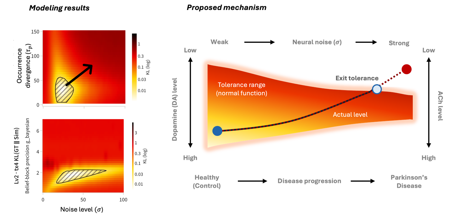
Moderate noise widens the tolerant regime for four mechanistically different parameters. Each block (τp, gβ, gbayesian, gI) maps the noise level σ (x-axis) against the parameter value (y-axis) at three rarities (N = 5, 10, 15; columns). The top row shows the Level-1 signed deviation on a diverging scale, where white means accurate; the bottom row shows the Level-2 KL divergence on a log scale, where pale means accurate. The hatched area on each Level-2 panel marks the 5% most accurate zone. For all four gains a band of moderate σ minimises both measures, and that accurate zone survives across rarities, so the noise correction does not hinge on any single dial.
Neural computation is noisy, so a mechanism that uses noise invites a biological reading: its sources, the neuromodulators that set the dials, and the diseases that move them.
Where σ comes from and why a moderate amount helps.
Vesicle release, channel gating and network fluctuations combine into one effective noise with a single amplitude [21]. That amplitude is our σ, applied to each unit's activation as in an earlier BCPNN sequence network [8].
Our inverted U is the signature of stochastic resonance: moderate noise lifts a weak signal, excessive noise drowns it [22]. The same optimum appears in single neurons, network synchrony, tinnitus and other internal-simulation models.
Cortical 1/f noise rises with age and tracks working-memory decline [18]; it is elevated in Parkinson's disease [19], and imprecise firing alone causes ataxia [26]. Noise that drifts upward slides off the optimum.
The model's parameters read as facets of one mechanism, each modulator distinct through its own receptors [27].
touches gβ and τp
Tonic dopamine sharpens the weight placed on the stored prior, the precision on priors [28, 29, 30], which maps onto gβ. It also sets how long the plasticity window stays open [31, 32], which maps onto τp.
touches gw (inside gbayesian), gI and ga
High cholinergic tone drives encoding from input; low tone releases the recurrent replay our simulation runs on [33]. One switch lowers gw, raises gI and relieves ga, but too little tone during learning corrupts training.
touches σ · the most tentative edge
Arousal plausibly sets the noise level, with detection best at intermediate arousal [34]. Noradrenaline is the candidate driver, and it may share a source with dopamine [35, 36].
| Parameter | Role in BCPNN | Modulator | Hypothesis | Prediction | Disease |
|---|---|---|---|---|---|
| τp | probability-trace timescale | DA | gates the plasticity window | slower timescale, slower learning | PD |
| gβ | prior belief (bias) | DA | intrinsic excitability | less DA, weaker prior | PD |
| gbayesian | internal-model precision | DA ACh | prior × evidence gain | moderate gain best | PD |
| ga | spike-frequency adaptation | ACh NE | suppresses sAHP and M-current | high ga frees stuck attractors | AD |
| gI | input / cue gain | ACh NE | gain on afferent input | low gain corrupts training | ADHD, AD |
| σ | replay-noise amplitude | NE | stochastic resonance from arousal-linked variability | fidelity peaks at moderate arousal | PD, ADHD |
Push the gains or the noise out of the tolerant band and rare events are mishandled.
Dopamine loss weakens the prior (gβ, τp): patients learn the odds yet fail to use them, over-weighting the rare [20], while subthalamic broadband noise rises with severity [19].
Cholinergic loss [37, 38] lowers gw and gbayesian, and blocking acetylcholine likewise over-weights rare locations [39]. Both push the simulation to over-represent rare events.